
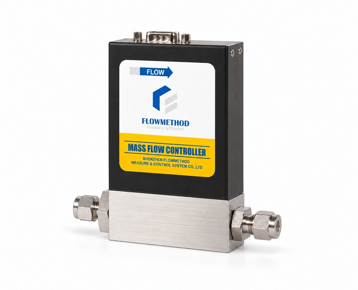
Many engineers open a thermal gas mass flow controller (MFC) or gas mass flow meter (MFM) for the first time, see a thin capillary and a few resistors, and ask a fair question: with so little hardware, how does it actually "count" gas flow? This article does not rush to the conclusion. It starts from the basic physics of convective heat transfer and peels the layers one by one — until you can walk the whole chain, "gas flows → the bridge temperature field changes → the servo loop computes the flow", completely and quantitatively, in your head.
Build the intuition first: thermal sensing measures heat carried away, not volume
Start with an everyday analogy. On a winter day, your hand feels warm in still air but cools noticeably when wind blows past it — the stronger the wind, the more heat it removes and the cooler your hand feels. A thermal gas mass flow meter uses exactly the same idea: put a heated winding in the gas path, the flowing gas "cools" it, and the degree of cooling is directly related to "how many gas molecules ran past it".
Two things are often confused and must be separated:
- Volumetric flow reads "how many liters of gas passed per unit time". But after being heated, the same volume holds fewer molecules: the volume is unchanged yet the amount taking part in the reaction drops — so a volumetric reading drifts with temperature and pressure.
- From the ideal-gas law ρ = pM/(RT), the mass m = ρV behind a fixed volume V falls as T rises; that is the inherent defect of volumetric sensing.
- Mass flow (the core of an MFC) corresponds directly to "how many gas molecules actually passed", and is essentially unaffected by temperature and pressure fluctuations.
The elegance of the thermal approach is precisely this: it measures the heat-dissipation rate of the platinum sensing windings, and when the gas composition is fixed, that rate has a stable relationship with mass flow. So a gas mass flow controller gives setpoints and readings that remain comparable across process temperature and pressure changes — which is why mass flow controllers are almost standard in ratio-sensitive processes such as gas mixing, coating and heat treatment.
Sensor structure overview: main path, capillary bypass and the thermal bridge
With the intuition in place, look at the hardware. The heart of a thermal gas mass flow meter is "main flow path + shunt bypass + thermal bridge". The overall structure and the temperature field it creates are shown below:
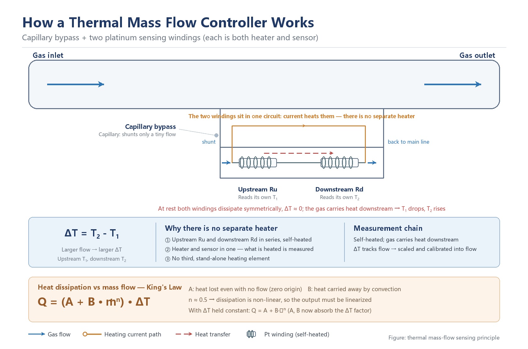
The main flow path (large bore) carries the bulk of the flow; a very small-diameter shunt channel — commonly a capillary bypass — is designed into it, letting only a tiny fraction pass through. Along the bypass, in the direction of flow, sit only two platinum (RTD) windings, forming the so-called thermal bridge:
- Upstream platinum winding Ru: sits in the front section of the bypass and heats itself as soon as current flows; what it reads is its own temperature T₁ after self-heating (the gas temperature plus the rise caused by its own current);
- Downstream platinum winding Rd: sits in the rear section, likewise self-heated, and reads its own temperature T₂ — which sits above T₁ by exactly the extra rise the flowing gas brought with it.
The key point: in this bypass-bridge structure there is no separate heater element. Both windings sit in series on one circuit — what is heated is exactly what is measured. Current makes them hot, and they report their own temperature rise. This pair of windings is then connected with a second bridge arm (two high-precision, temperature-stable resistors) to form the Wheatstone bridge described in the section on the Wheatstone bridge.
Why not just insert the bridge into the main path and instead route through a bypass? Three engineering reasons:
- Low pressure drop: the bypass shunts only a tiny flow, so the main path is almost unobstructed — critical for low-pressure conditions;
- Pollution resistance: the high main-path velocity sweeps dust and oil away, while the sensitive temperature elements hide safely inside the thin bypass;
- Controllable range: the bypass scales "large flow" down to "small flow" before measurement, widening the turndown ratio while protecting the fragile sensing structure.
At rest, both windings dissipate heat symmetrically upstream and downstream, so the upstream-downstream temperature difference tends toward zero. Once gas flows, it carries heat toward the downstream side and breaks the symmetry — the faster the flow, the hotter the downstream side and the larger the temperature difference. This "temperature difference changes monotonically with flow rate" is the entire physical starting point of thermal measurement.
From convective heat transfer to King's law: what is the relation between temperature difference and flow
Let me try to explain how to turn "the temperature difference seems to vary with flow" into a quantifiable, calibratable relation. When gas crosses a platinum winding, the convective heat transfer is governed by the Nusselt number: Nu = h·D / k = A₀ + B₀·Reⁿ where h is the convective heat-transfer coefficient, D the winding diameter, k the gas thermal conductivity, Re = ρuD/μ the Reynolds number (ρ density, u velocity, μ dynamic viscosity), and A₀, B₀, n empirical constants. The heat transferred is Q = h·Aₛ·ΔT (Aₛ winding surface area, ΔT winding-surface-to-gas temperature difference). Substituting ṁ for Re (Re ∝ ṁ), and then that into Q = hAₛΔT, yields the core empirical equation of thermal measurement — King's law: Q/ΔT = A + B·ṁⁿ The strict form keeps the temperature difference: the heat loss Q is proportional to ΔT, and it is the coefficient that depends on flow. Under constant-temperature-difference control ΔT is held fixed, so the equation reduces to Q = A + B·ṁⁿ — at that point A and B have absorbed the fixed ΔT factor. — and it is exactly along this line that the two implementations in the next section split the job: hold ΔT fixed and measure power, or hold power fixed and measure ΔT. Read the physical meaning term by term: the A term is the heat that must be dissipated even with no flow (natural convection and wall-conduction losses) — it is exactly the origin of the zero point; the B·ṁⁿ term is what the gas convection carries away, and the larger the flow, the more dominant this term; the exponent n is often near 0.5, meaning dissipation and flow are not simply linear — which is the root reason "linearization is mandatory later". To be clear: King's law is an empirical calibration relation, not a strictly derived closed-form solution from first principles. Real sensors also have radiation, the element's own heat capacity, and bypass flow-field non-idealities. So every thermal gas mass flow meter must be calibrated with a reference gas in the factory, which fixes A, B and n into its conversion table. This is also why meters "of the same principle" from different MFC manufacturers may differ in accuracy and linearity — the calibration and compensation algorithms sit below the iceberg.
From the temperature-difference signal to a flow reading: two common implementations
The bridge measures an upstream-downstream temperature difference, and the circuit turns it into an electrical signal — that signal, once amplified and converted against calibration, gives the mass flow. So at the level of principle one sentence suffices: the temperature difference is an intermediate quantity, and flow is the result computed from the temperature-difference signal. In engineering there are two common implementations with different traits, both doing the same job:
Constant temperature difference: a servo loop holds the temperature difference at a setpoint; whatever heat the gas removes is replaced as power, so the power fed in maps one-to-one to flow (the diagram below shows such a loop). It gives fast response and a stable zero, suited to closed-loop control with frequently changing setpoints.
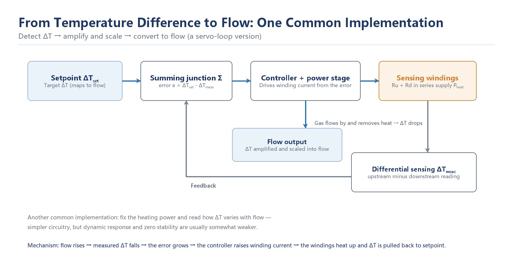
Constant power: the power is held fixed and the temperature difference is read directly and converted back into flow; the closed loop is dropped and the circuit is simpler, but dynamic response and zero stability are usually somewhat weaker.
Both deliver a mass-flow reading; the difference is an implementation trade-off, not a question of "which is more accurate". For selection, calibration quality and compensation algorithms matter more than the name of the control scheme.
From bridge to output: from the Wheatstone bridge through flow linearization and conditioning to the output
The sensor body is usually not a set of unrelated resistors, but is wired as a Wheatstone bridge. In the common arrangement, the upstream and downstream RTD windings are connected in series to form one bridge arm, while the other arm is made of two high-precision, temperature-stable resistors in series; the two arms sit in parallel across the excitation supply, and the voltage difference between their midpoints is taken as the output. The gas flow changes the resistance of the RTD windings, and the bridge then outputs a weak voltage proportional to the temperature difference.
One practical issue has to be handled: two RTDs of the same type still differ slightly in resistance, so a zero offset remains. This is normally taken out by a small trim potentiometer in the middle of the RTD arm — adjusted at factory calibration to pull the two midpoint potentials to the same level, so the output is zero at zero flow. That is also why field zeroing and factory zeroing are separate jobs: the factory deals with component consistency, while field zeroing deals with the offset introduced by the gas line and the installation.
The chain from here decides whether a meter is "good to use". Step one, instrumentation amplification: the bridge output is a millivolt-level weak signal, first boosted by an instrumentation amplifier that also rejects common-mode temperature drift. Step two, temperature compensation: when ambient temperature changes, the RTD base resistance also drifts, so another temperature-sampling path compensates, otherwise the reading follows the room temperature. Step three, linearization: recall King's law from the section above — flow and output are not linear, so the controller runs an inverse function or a lookup algorithm to "straighten" the nonlinear curve, making the 4-20mA / 0-5V output linearly correspond to the real flow. Step four, digital interface: the linearized result goes through ADC and MCU, then outputs as 4-20mA, 0-5V, or up to a host computer or PLC via RS-485 / digital protocol.
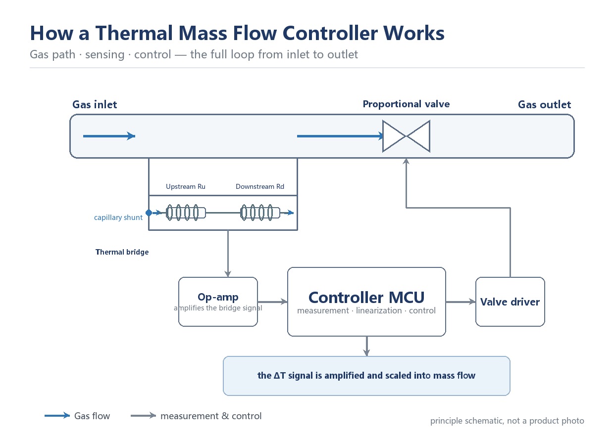
At this point the chain "gas flows → bridge temperature difference → bridge voltage → amplify and compensate → linearize → standard signal" is fully closed. The setpoint you adjust is the target flow: the controller compares the flow measured at the bridge with the setpoint and then drives the control valve to change the flow area.
Put that chain back into a complete instrument and you get the loop from gas path to valve control. Gas enters through the inlet, passes the thermal bridge sensing section and leaves through the outlet past a proportional valve. The bridge signal is amplified by an op-amp and taken to the controller MCU, which performs the measurement, the linearization and the control calculation, then drives the valve through the driver stage.
The gas conversion factor: why the reading changes with a different gas
All the relations above hide one premise: the gas composition is fixed. But B and n in King's law directly depend on the gas specific heat cₚ and thermal conductivity k — those differ between gases, so the same bridge behaves differently for nitrogen versus argon.
Hence the gas conversion factor (also called K factor). The device is first calibrated on a reference gas, almost always nitrogen (N₂). When you switch to argon, carbon dioxide or methane, the reading must be converted by the corresponding factor. The conversion is not a guess — it is an equivalent relation computed from the weighting of each gas's cₚ, k and density within the King's-law model.
Strictly speaking, B and n are not the only gas-dependent terms: the A term (heat loss at zero flow) and the conversion factor itself also shift with gas properties — change the thermal conductivity and the specific heat capacity and both the zero baseline and the conversion relation move with them. B and n are the two most directly affected, but not the only ones.
For multi-gas users, this is the lifeline: whether you need to recalibrate after switching gas depends on whether the manufacturer's gas library contains that gas's factor; how accurate the factor is depends on how deeply the model covers each gas's properties — rarefied gases and mixtures often carry larger errors; and even with a factor, when the actual condition (temperature, mix ratio) deviates from calibration, a residual conversion error remains to be corrected on site.
So when selecting, "which gases are supported, how the factor is given, and the conversion error band" should be asked as hard requirements alongside range and accuracy.
Accuracy and error sources: why the same meter can still read wrong
Only with the principle understood can you read what those accuracy specs on a datasheet actually mean. Thermal-meter errors mainly come from the following classes:/n
- Zero drift: the bridge slowly shifting its no-flow baseline under thermal stress, contamination or temperature cycling, showing up as an overall offset in the low-flow range.
- Span drift (a drift of the full-range scale): comes from winding aging or a changed calibration reference, causing proportional error across the full range.
- Linearity error: appears when King's-law nonlinearity is not fully compensated, so the mid-range deviates more than the ends.
- Temperature effect: added error from incompletely compensated ambient-temperature change (usually given as ±%FS/℃).
- Pressure effect: although mass flow is measured, at high pressure the changed gas density and heat-transfer coefficient still introduce a small deviation.
- Repeatability: measures the scatter of repeated measurements under identical conditions, reflecting the servo loop and noise level, and is usually better than the accuracy.
These often have to be read separately: a meter can be "excellent repeatability but mediocre absolute accuracy" (good for ratio closed loops), or "high accuracy but large temperature drift" (needs a thermally stable environment). When selecting, pick the item directly relevant to your duty rather than staring at a single "accuracy %".
Dynamic response: why the reading does not follow instantly after a flow step
Thermal measurement works on thermal balance and is essentially a thermal-inertia system; the response can be approximated by a first-order lag: output(t) ≈ input·(1 − e^(−t/τ)) where τ is the thermal time constant, set by the winding's heat capacity, dissipation rate and bypass structure. Two consequences follow: first, response time — how fast the output catches up after a flow step; the servo-loop implementation is usually faster because it actively compensates. Second, warm-up: after power-on the bridge must move from room temperature to a stable thermal balance; putting it into service before it is thermally settled is reading on a drifting zero, so adequate warm-up is generally required before use — follow the manual for the specific instrument (see the field section below). This is also why thermal meters are unsuited to "ultra-high-speed pulsating flow" — their strength is steady/slowly-varying small-flow precise control, not catching transient spikes.
Sensor taxonomy: "thermal" itself has different implementations
Speaking of "thermal principle", it is easy to mistake it for a single structure. This taxonomy can be read along two dimensions: where the sensor sits in the gas path, and the form of the sensing element. By sensor location there are mainly two families:
- Bypass / split-flow (capillary): the main line of this article, the bridge hides in a thin bypass, the main path has low pressure drop, better suited to low-pressure gas. Flowmethod FL-802 / FL-803 / FL-805 / FL-807 and CM-802LD / CM-803LD / CM-805LD / CM-807LD belong here.
- In-line / insertion: the bridge sits directly in the main path or pipe center, saving the bypass, simpler in structure, but with higher pressure drop and contamination risk; common for large bore or special media.
By sensing element form there is hot-wire (thin metal wire, extremely fast but fragile), hot-film (film on a substrate, more durable), and a class of MEMS thermal sensors, where the sensing element is made as a small chip-scale package placed in direct contact with the gas path — this drops the wire-winding or coating process, gives fast response and a compact footprint, but raises the demands on manufacturing consistency and contamination protection. This taxonomy explains the "bypass vs in-line", "hot-wire vs hot-film" and "MEMS" differences you see in vendors' datasheets.
| Aspect | Bypass / split-flow | In-line / insertion |
|---|---|---|
| Main-path pressure drop | Low (the bypass takes only a tiny fraction) | Higher (the probe sits directly in the main line) |
| Contamination resistance | Better (the sensing element hides inside the thin bypass) | Worse (exposed to the main stream) |
| Structural complexity | Needs a bypass and a capillary | Simpler |
| Typical use | Low pressure, small flow, high-accuracy duties | Large bore, where pressure loss is acceptable |
Field engineering points: warm-up, zeroing and contamination
With the principle clear, in the field a few actions directly decide whether the reading is accurate — and they lie at the root of many "broken device" complaints.
Adequate warm-up: the bridge works on steady thermal balance; after power-on, warm up for 15 minutes or more (follow the manual) so the upstream-downstream thermal field stabilizes; putting it into service before it is thermally settled is reading on a drifting zero.
True no-flow zeroing: zeroing must be done after closing the valve, confirming there is genuinely no flow in the line, and with temperature stable; zeroing with flow present writes the line problem into the zero point, and nothing will calibrate correctly afterward.
Contamination sensitivity: oil, particles or condensate on the bridge or capillary wall change local thermal conduction and the flow field, showing up as zero drift and small-flow inaccuracy; filter and dry ahead of the instrument on low-quality gas sources.
After switching gas or long idle: re-check the zero before starting the formal process.
These look like operational details, but they are the "balance cost" thermal principle must pay in engineering — you benefit from low pressure drop, small-flow capability and no moving parts, so you must respect the rules on thermal balance and cleanliness.
Flowmethod FL and CM series: thermal principle in engineering
Shenzhen Flowmethod Measure & Control Systems Co., Ltd. (Flowmethod) FL-802 / FL-803 / FL-805 / FL-807 series gas mass flow controllers and CM-802LD / CM-803LD / CM-805LD / CM-807LD series integrated-display mass flow controllers are an engineering realisation of the thermal mass flow measurement principle described above, a gas flow controller built for low-pressure duty. In the nitrogen-equivalent ranges published on the website, FL-802 covers 0–10 SLPM, FL-803 10–50 SLPM, FL-805 50–200 SLPM and FL-807 200–1000 SLPM; the CM series covers the same ranges model for model (the exact structure and range of each model are given in its own datasheet), and they offer configurations such as integrated-display gas mass flow controllers, split type and digital communication for easy connection to PLC or a host computer.
It must be stressed: thermal is only the "measurement principle"; under the same principle, manufacturers differ widely in structural process, control algorithm and production-calibration capability — and those below-the-iceberg parts are what really decide how well it works in your field. When doing mass flow controller selection, ask clearly about "which gases are supported, how the conversion factor is given, communication and control modes, and after-sales calibration", then decide against your actual working conditions — a flow meter with a handsome spec sheet is not yet a reliable flow meter in the field.
For selection, product documentation or technical enquiries, contact Shenzhen Flowmethod Measure & Control Systems Co., Ltd.:
Contact: Mr. Dou | Tel: +86-18038183381
Email: doufeijin@hotmail.com | Website: www.flowmethod.net