
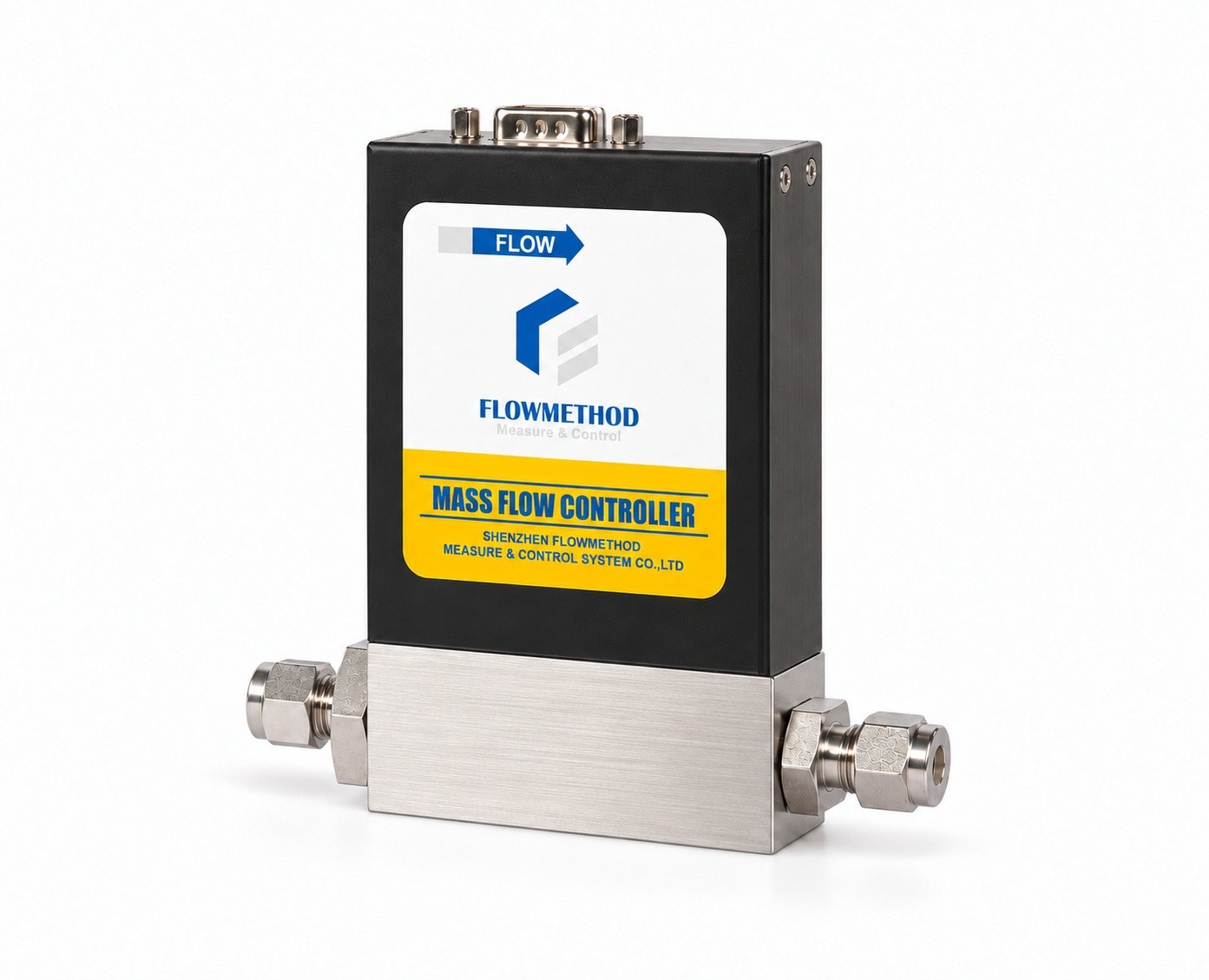
Order a gas flow controller with methane as the medium and 100 SLPM as the flow. The instrument is calibrated against nitrogen (or air) on the production bench, so that 100 SLPM first has to be converted into an equivalent flow of the calibration gas, and the number that does the conversion is the gas conversion factor (GCF). This article walks the whole chain: why the conversion exists, how the factor is calculated, how a mixture is weighted, and how the range is chosen once the equivalent flow is known. It closes with two complete worked examples — a single gas and a gas mixture — that you can reproduce on paper with one table of physical properties. This is the step most often skipped in mass flow controller selection, and the hardest one to repair after delivery.
1. Three assumptions hidden in a single order line
Start by asking what "100 SLPM of methane" actually presupposes. Nitrogen or air is only the calibration gas; the delivered medium is methane itself. When you order a methane unit, the nameplate, the range, the setpoint and the display are all written in methane. Nitrogen (or air) is merely the gas that flows on the calibration bench, where the manufacturer establishes the curve against an equivalent flow derived from methane. A calibration bench has to generate standard flow that is stable, traceable and repeatable in production, and nitrogen satisfies nearly all of it: inert, non-flammable, non-corrosive to sensors and seals, easy to keep pure, with complete property data and low cost. Air serves as an equivalent reference in some cases and differs from nitrogen by only about 0.1% to 0.5%: dry air at 21% O₂ and 79% N₂ lands within roughly 0.1% to 0.2%, while air carrying water vapour and CO₂ raises the volumetric heat capacity slightly and can reach the 0.5% order. Engineering-wise the two can be treated as equivalent, but when accuracy matters or the supply fluctuates, the reference gas still belongs in the agreement. The reverse case explains why this convention exists at all: in semiconductor and photovoltaic processes, many media — silane, phosphine, ammonia, hydrogen chloride, tungsten hexafluoride — are pyrophoric, acutely toxic or aggressively corrosive, and cannot be run through a calibration bench across the full range. The industry answer is to establish the production reference on nitrogen and convert every other gas into an equivalent flow, or to calibrate the unit on the actual process gas and ship it that way.
SLPM means standard litres per minute, and it is a molar flow. A mass flow controller (MFC) is called a mass flow device because its reading does not drift with the temperature and pressure at the point of use, yet the industry expresses that reading as a standard volumetric flow, because at reference conditions the gas density is a constant and standard volume maps one to one onto mass. So 100 SLPM means "100 litres per minute, referred to the reference conditions" — independent of whether the line is at 2 bar or 25°C at that moment.
"Standard conditions" must state the reference temperature and pressure, or the number can be off by more than 7%.
- Standard conditions are 101.325 kPa(a) at 0°C, giving a molar volume of 22.414 L/mol;
- Normal conditions are 101.325 kPa(a) at 20°C, giving a molar volume of 24.055 L/mol.
The same physical stream is 100 SLPM on the 0°C basis and 107.3 SLPM on the 20°C basis. The ratio is 293.15/273.15 = 1.0732, or 7.32%. That deviation contains no instrument error at all; it comes purely from the definition of the reference temperature. This is why a technical agreement has to carry the medium, the flow value and a line such as "reference conditions: 0°C / 101.325 kPa(a)" together. Without it, two suppliers or two calibration benches will deliver devices with different actual gas quantities against the same order.
Put the three together and what you owe the manufacturer is not "methane, 100 SLPM" but: reference conditions, calibration gas, the actual flow of the target medium at those conditions, and the equivalent flow in the calibration gas. There is no universal default for reference conditions. Practice differs by industry and by manufacturer, and all three of 0°C, 20°C and 25°C are in real use — semiconductor equipment and most instrument makers favour 0°C, parts of the process industries use 20°C, and environmental monitoring often shows 25°C. Confirm it before you order rather than letting a "default" decide. The worked examples below use 0°C / 101.325 kPa(a) purely so the arithmetic can be followed, not as an industry convention.
2. Why the conversion is unavoidable: the sensor measures heat carried away
The need to convert follows from the measuring principle, not from paperwork. Take the most common thermal mass flow controller: a capillary sensing channel is split off the main path, with heating and temperature-sensing elements wound on the outside. As gas passes, it carries heat from the upstream side to the downstream side and establishes a temperature difference. At steady state the energy balance reads "heating power = heat convected away by the gas + losses to the tube walls and ambient": P = ṁ × cp × ΔT + P_loss.
Here ṁ is mass flow and cp is specific heat at constant pressure. Converting mass flow to standard volumetric flow Q gives ṁ = ρ × Q, with ρ the density at reference conditions, so the quantity the sensor is really sensitive to is P — P_loss ∝ (ρ × cp) × Q. What a given output signal corresponds to is the product of volumetric heat capacity and volumetric flow; flow alone does not determine it. Change ρ or cp and the same Q produces a different signal, so the reading must be converted.
One step further yields a conclusion that is counter-intuitive and genuinely useful. For an ideal gas, ρ = M / V_m with M the molar mass and V_m the reference molar volume, while specific heat cp = Cp,m / M with Cp,m the molar heat capacity at constant pressure. Multiplying the two cancels the molar mass: ρ × cp = Cp,m / V_m. Within the ideal-gas approximation, the sensitivity of a thermal sensor is governed mainly by the molar heat capacity at constant pressure, not by molecular weight directly. Monatomic gases (Ar, He) have only translational degrees of freedom, with Cp,m ≈ 20.8 J/(mol·K); diatomic gases (N₂, O₂, H₂, CO) sit near 29 J/(mol·K); polyatomic molecules add rotational and vibrational modes, giving about 37 J/(mol·K) for CO₂ and 35.7 J/(mol·K) for CH₄. The larger the molar heat capacity, the more heat a given flow carries away, the more sensitive the sensor, and the smaller the actual flow needed to produce the same signal. That is exactly why argon and helium end up with factors above 1 while methane, propane, carbon dioxide and sulphur hexafluoride sit clearly below it. Remembering this physical thread is worth more than memorising a factor table.
Theory alone does not explain everything, though. A real sensing channel also involves thermal conductivity, viscosity, the Prandtl number, the bypass split ratio and wall losses, so the engineering expression keeps a molecular structure factor N (also called a structural correction factor), taken from empirical bands for monatomic, diatomic, triatomic and polyatomic molecules. The gas conversion factor is a product of physical properties and a specific sensor geometry, which makes it a device-dependent quantity — copying another brand's table inevitably imports extra error. A second technology, the laminar differential-pressure mass flow controller, passes the gas through a laminar element and derives volumetric flow from the pressure drop by the Hagen-Poiseuille relation Q = (π × r^4 × Δp) / (8 × μ × L). There the governing property is dynamic viscosity μ, and the instrument then applies absolute pressure, temperature and compressibility corrections to refer the volume to standard conditions. The "gas factor" of such a device is entirely different from a thermal one, and may even order the same gases differently. A Coriolis mass flow meter measures mass directly and is in principle indifferent to gas species. So before using any general gas factor table, confirm which measuring principle it belongs to — applying a thermal table to a laminar differential-pressure instrument is one of the most common and hardest-to-trace error sources on site.
3. How the gas conversion factor is calculated: C = 0.3106 × N / (ρ × cp)
The expression used across the domestic thermal MFC industry matches the definition of the Gas Correction Factor: C = 0.3106 × N / (ρ × cp), where ρ is the density at standard conditions (0°C, 101.325 kPa) in g/L, cp is the specific heat at constant pressure in cal/(g·°C), and N is the molecular structure factor. The constant 0.3106 is simply the ρ × cp of the nitrogen reference: 1.250 g/L × 0.2485 cal/(g·°C) ≈ 0.3106. Nitrogen therefore returns C = 1.000, and the whole table is by construction a ratio against nitrogen. The empirical bands for N are:
| Structure | Examples | N |
|---|---|---|
| Monatomic | Ar, He | 1.01 |
| Diatomic | N₂, O₂, H₂, CO | 1.00 |
| Triatomic | CO₂, N₂O | 0.94 |
| Polyatomic | CH₄, NH₃, C₃H₈ | 0.88 |
Different references give the same factor as 1.030 / 1.000 / 0.941 / 0.880 or as 1.01 / 1.00 / 0.94 / 0.88, with a small discrepancy in the monatomic band; products also differ because sensor geometry and empirical calibration data differ, so factor tables were never meant to be identical. That is the technical reason — not a courtesy phrase — for "use the table in the manual of the product you are buying". The table below is recalculated from the ideal-gas molar volume of 22.414 L/mol together with each gas's molar mass and specific heat, to check that the formula and published gas conversion factor tables agree (ρcp here is ρ × cp in cal/(L·°C)):
| Gas | ρcp | N | C |
|---|---|---|---|
| N₂ | 0.3106 | 1.00 | 1.000 |
| O₂ | 0.3127 | 1.00 | 0.993 |
| H₂ | 0.3076 | 1.00 | 1.010 |
| Ar | 0.2217 | 1.01 | 1.415 |
| CO₂ | 0.3947 | 0.94 | 0.740 |
| CH₄ | 0.3801 | 0.88 | 0.719 |
Values are shown to three decimals; densities come from the 22.414 L/mol molar volume and the molar masses. Measured densities in published data differ slightly because of real-gas compressibility, which is why common tables disagree in the last digit by a few percent. The recalculated values match the general table item by item (CH₄ 0.72, Ar 1.42, CO₂ 0.74, H₂ 1.01, O₂ 0.99), which confirms the expression is self-consistent and can be checked independently. The table has firm applicability limits. The ρ and cp above are values for near-ambient temperature and pressure, roughly 0 to 50°C and around 0.1 MPa. At higher pressure, away from ambient temperature, or near saturation and the critical region, both ρ and cp move with the operating point and must be recomputed from an equation of state with the compressibility factor Z; a table of atmospheric-pressure factors cannot simply be applied. Mixtures at high pressure deserve particular care: components have different Z values, the error of a linear overlay by volume fraction is amplified by pressure, and the honest route is to compute real densities component by component and then weight them, or to measure directly at the operating conditions.
With C in hand, the two directions have to be kept apart. This is where the field most often multiplies the wrong way:
- From a reading to actual flow: Q_actual = Q_reading × C. This presumes the unit is still nitrogen-calibrated and no gas has been selected or factor written into it — once switched internally, the reading is already target-gas flow and multiplying again double-converts. A nitrogen-calibrated unit on argon reading 100 sccm passes 141.5 sccm.
- From a target flow to the calibration equivalent, or to a setpoint: Q_equivalent(N₂) = Q_target / C. For 100 SLPM of methane the nitrogen equivalent is 100 / 0.72 = 138.9 SLPM.
The first direction answers "I already own the instrument, what is it really flowing"; the second answers "what equivalent flow must production calibrate against". Every calculation in this article uses the second. The equivalent-calibration loop closes as follows: the manufacturer runs nitrogen on the bench and, for each target-gas flow point, uses the corresponding nitrogen equivalent to establish the curve between sensor output and flow; the instrument then converts through the target gas factor so that display, setpoint and nameplate all read the target gas. What the customer receives is a range and a reading in the target gas, while the curve itself was built in a nitrogen loop up to an equivalent-flow ceiling. Whether the conversion happens in the instrument or in a host system depends on the model: some allow gas selection and factor entry on the panel or over digital communication, others offer only analog signals and leave the conversion to the PLC. The manual for that model governs.
The accuracy boundary has to be stated as clearly, or the conversion gets treated as a universal remedy. Industry technical literature typically notes that with a GCF the accuracy of the flow reading may change by about ±5%, while repeatability stays at ±0.2% FS; where linearity and accuracy must improve, calibrating on the process gas itself, or on a substitute with similar properties, is the recommended route. In other words, the conversion buys usability, not precision. An error budget should carry at least four items: the empirical spread of the factor itself, the accuracy basis of the calibration, the reference conditions and supply purity, and the non-linearity and zero drift of the sensor at low flow. If the process tolerance is tighter than ±2%, there is only one sound conclusion: state the actual medium on the order and calibrate the unit on that gas at the factory.
4. Gas mixtures: weight by volumetric heat capacity, never average the factors
A mixture of fixed composition can indeed be converted, but its gas conversion factor holds a trap that is easy to fall into. The factor of a mixture cannot be a weighted average of the component factors — what can be weighted is the sensible heat each component carries, and the factors themselves are not additive. The correct form is C_M = 0.3106 × Σ(a_i × N_i) / Σ(a_i × ρ_i × cp_i), where a_i is the flow share of component i (mole fraction, summing to 1), N_i its molecular structure factor and ρ_i × cp_i its volumetric heat capacity.
Why can the factors not simply be averaged? Because only heat is additive. Section 2 showed that the sensor output is proportional to the product (ρ × cp) × Q; the heat powers carried by the components of a mixture add up, so the total signal is proportional to Σ(a_i × ρ_i × cp_i) × Q_total. Weighting the denominator by volumetric heat capacity is a physical necessity, whereas averaging the factors performs the division too early and does not hold mathematically. The numerator must in turn be weighted by each component's structure factor N_i for the expression to be complete. How far apart the two results sit is quantified in the worked example in Section 7 — with components of very different properties the deviation reaches the 7% order, enough to ruin a gas mixing experiment.
The expression carries several preconditions, and missing any one of them rules it out:
- The composition must be fixed. If the mixing ratio moves with time there is no single mixture factor; the standard industry wording is that a gas mixture whose mixing ratio is not fixed has no calculable conversion factor.
- The components must not react, releasing or absorbing heat. Reaction heat lands directly on the sensor's heat balance, while the expression accounts only for sensible heat.
- No condensation and no significant adsorption. With water vapour, heavy hydrocarbons, ammonia or hydrogen chloride, components can be lost in the line or in the sensing channel, so the composition reaching the sensor is no longer the cylinder's nominal composition.
- Near-ideal gas behaviour, within the linear band of the sensor. At high pressure the density needs a compressibility correction; large molecules and strongly polar gases also produce cross terms that make linear superposition inaccurate.
- Factors taken from the same device and the same property basis. Assembling a mixture denominator from another basis's single-gas factors mixes two empirical systems.
So what happens when the composition has to change? The engineering answer is rarely "find a factor that varies" but rather a change of architecture: give each pure component its own MFC, control it separately, and mix downstream. Each instrument then sees one known gas, the ratio is set by the individual setpoints, it can be changed online at will, and every applicability condition for a mixture factor is bypassed. That is why a gas mixing system is normally built as a multi-channel arrangement — it is an architectural choice, not an admission that the numbers cannot be worked out. A single mixture factor pays off only where composition is constant, the gas path must stay simple and moderate accuracy is acceptable.
5. After the equivalent flow: how to size the range
The equivalent flow is only the numerator. Sizing a mass flow controller also means looking at the upper limit, the lower limit and the control capability, plus one rule about rounding — four items, none optional. First, though, the general principle: choose the range by rounding the customer's actual flow of the target medium; the equivalent flow is not used to pick a range. The full scale is rounded from the actual service flow of the target gas (for example, if the maximum is 120 SLPM, a 130, 140 or 150 SLPM full scale all cover it, and which one you take depends on the normal point and the minimum point), and the nameplate, setpoint and interface are all written on that basis. The equivalent flow in the calibration gas is a production-calibration and internal-setting parameter and takes no part in range selection. Round from the equivalent flow instead and the range delivered to the customer is a number that only holds after conversion, which makes field setup, verification and spare-part replacement unintuitive — which is precisely why the rule is to round from the customer's flow, not from the equivalent. This is the practical backbone of any mass flow controller selection guide.
Upper limit and rounding: do not push the maximum into full scale, and leave a margin you can calculate. A normal flow between 20% and 80% of full scale is the selection basis Flowmethod has always used. But there is no fixed coefficient to apply: starting from the design maximum, one step or two steps up may both hold, and the choice is settled by the normal point and the minimum point together, with cost-effectiveness as a third consideration — different steps sometimes land in a different product family, and a range only slightly larger can push the cost up a step. In selection we normally start from where the customer actually spends most of the time, keep the normal point inside 20% to 80%, then check margin against the peak and controllability against the minimum; where several steps all pass, take the smallest, and do not buy an extra step for an occasional peak. More margin is not automatically better either: if the normal point is pushed below 40% of full scale, that step has been paid for and not used.
Lower limit: the equivalent flow at the minimum condition must not fall near the control floor (minimum controllable flow). This is the constraint more often overlooked than the upper one. If accuracy is stated as full scale accuracy, ±1% FS, the relative error is ±5% at 20% FS and ±10% at 10% FS; if it is specified as ±1% RD (percentage of reading), the absolute error at low flow shrinks with the reading instead. The same instrument therefore permits a completely different minimum flow depending on the accuracy basis. Zero drift, seat leakage and setpoint resolution are absolute quantities as well, so their share grows as flow falls. "Buy a bigger range to be safe" is the wrong instinct: the larger the range, the worse the low-flow segment performs for the money.
Control capability: inside the range does not mean under control. An MFC is a closed loop and needs enough upstream-to-downstream differential pressure to drive the valve; with insufficient inlet pressure, excessive back pressure or heavy line loss, the valve can open fully and still not reach the target flow. Sizing therefore has to check the inlet absolute pressure, the outlet back pressure and the required pressure ratio at maximum flow together — a constraint orthogonal to range. Multiple gases in rotation: convert each one and take the intersection. When a single controller must pass several gases in turn, convert each gas's maximum and minimum actual flows into equivalents of the calibration gas to verify the instrument's physical ceiling and controllable floor; the range is still rounded from the actual flow of the primary gas. If the converted span exceeds the usable span of that instrument, the conclusion is separate control paths, calibration per primary gas, or a model with a wider usable span. Usable span cannot be estimated from marketing copy: Flowmethod thermal products are specified over 1% to 100% FS, but with accuracy expressed in %FS, a ±1% FS unit carries ±100% relative error at the 1% FS point, so the practically usable metering span is usually only 5:1 to 10:1; laminar differential-pressure and Coriolis designs can be built wider. A combination such as 2 SLPM of nitrogen purge plus 30 SLPM of propane main flow, an order of magnitude apart, is simply hard for one range to serve.
Finally, write the ordering information list in full: medium and purity, whether the composition is fixed, reference conditions (agree them in writing; 0, 20 and 25°C are all in use), calibration gas, maximum, normal and minimum actual flow, range step (rounded from the target gas's actual flow), converted equivalent flow (for the manufacturer to verify calibration capability), accuracy basis (%FS or %RD), inlet and outlet pressure, signal type, and whether calibration on the actual gas is required. These eleven items in a technical agreement are worth far more than arguing later about whether the instrument was accurate.
6. Worked example 1: ordering 100 SLPM of methane
Given: the process needs 100 SLPM of CH₄; reference conditions follow this article at 0°C / 101.325 kPa(a) (example setting only); production calibration runs on N₂ (or air) equivalent flow; normal flow 100 SLPM, process excursion ceiling 120 SLPM, minimum operation 20 SLPM; accuracy budgeted at ±1% FS. The range is rounded from the customer's actual methane flow, and the example takes a 130 SLPM (CH₄) full scale. The example range and accuracy basis serve the calculation only and represent no specific model; the datasheet of the model actually selected governs. Step 1, the factor. CH₄ is polyatomic, so N = 0.88; with ρ = 0.7158 g/L and cp = 0.531 cal/(g·°C), ρcp = 0.3801, giving C = 0.3106 × 0.88 / 0.3801 = 0.2733 / 0.3801 = 0.719 ≈ 0.72.
Step 2, convert to the nitrogen equivalent. The result belongs to production calibration, not to the customer's range. Q_equivalent = 100 / 0.72 = 138.9 SLPM(N₂). Likewise the 120 peak corresponds to 166.7 SLPM(N₂) and the 20 minimum to 27.8 SLPM(N₂); the selected 130 SLPM(CH₄) full scale corresponds to 130 / 0.72 = 180.6 SLPM(N₂). That 180.6 has to be checked separately against the calibration bench's capability: calibrating a 130 SLPM methane unit requires the nitrogen loop to hold 180.6 SLPM or more, which involves the reference meter's range, the branch bore and the pressure loss. It is a calibration-capability check item — neither the customer's range nor a basis for choosing a step. The manufacturer calibrates against these equivalent points, while the nameplate and setpoint delivered to the customer still read 0 to 130 SLPM of methane.
Step 3, fix the step from the customer's actual flow. With a maximum of 120 SLPM(CH₄), 130, 140 and 150 all cover the peak. This customer runs mostly at 100 SLPM, so a 130 SLPM(CH₄) full scale is taken: the normal point at 100 / 130 = 76.9% sits in the upper-middle of 20% to 80%, and both margin and cost efficiency are sound; the peak at 120 / 130 = 92.3% is usable with a narrow margin, acceptable because the excursion is short-lived; the minimum at 20 / 130 = 15.4% has dropped below 20% and is handled separately in Step 4. If the customer sat at 120 for long periods and only passed through 100 occasionally, 140 or 150 would be the safer choice (120 / 150 = 80.0%), at the cost of pushing the normal point down to 66.7% and making the low-flow segment worse. There is no single correct step; the difference is how you weigh the normal point against the minimum — which is exactly why rounding has to be judged by a person rather than by a coefficient.
Step 4, check the upper and lower limits. The three conditions occupy 15.4% (minimum 20 SLPM CH₄), 76.9% (normal 100) and 92.3% (peak 120) of the 130 step. A minimum of 15.4% is below 20%: at ±1% FS the absolute error is ±1.3 SLPM(CH₄), which is about 6.5% relative at 20 SLPM — if that segment matters to the process, give it a small dedicated controller; carrying it on a large range costs more in error than it saves in hardware. Step 5, setpoint conversion (analog models). With 0-5 V spanning 0-130 SLPM(CH₄), a setpoint of 100 SLPM is 76.9% of full scale, so the output is 5 × 0.769 = 3.85 V; on 4-20 mA it is 4 + 16 × 0.769 = 16.31 mA. Digital models do this internally once CH₄ is selected or the factor written on the panel or host.
Step 6, error budget and conclusion. The factor conversion itself contributes about ±5%; adding the calibration accuracy, the reference-condition basis and supply purity, the uncertainty on 100 SLPM lands around ±5 SLPM. If the process only needs the gas quantity to be roughly right, the conversion is entirely adequate; if the process is held within ±2%, the conclusion has to be written the other way round: do not convert, order "100 SLPM methane, calibrated on methane at the factory" and let the factor return to 1. We normally advise calibrating on the actual gas whenever the tolerance is tighter than ±2%, rather than using a converted value to hold a tolerance.
7. Worked example 2: a three-component mixture at 60 SLPM
Given: a gas mixing application uses a fixed-composition mixture of Ar 50%, CH₄ 30% and H₂ 20% (mole fraction) at a total of 60 SLPM, with the same reference conditions as Example 1; production calibration runs on N₂ equivalent flow; normal 60 SLPM, peak 80 SLPM, minimum 10 SLPM, accuracy budgeted at ±1% FS. The composition is for demonstration only; any hydrogen-bearing or flammable medium requires seal materials, hazardous-area classification and safety boundaries to be settled first. Step 1, list each component's volumetric heat capacity and structure factor (ρcp from the recalculated table in Section 3):
| Component | a | ρcp | N |
|---|---|---|---|
| Ar | 0.50 | 0.2217 | 1.01 |
| CH₄ | 0.30 | 0.3801 | 0.88 |
| H₂ | 0.20 | 0.3076 | 1.00 |
Step 2, calculate numerator and denominator separately. Σ(a_i × N_i) = 0.50×1.01 + 0.30×0.88 + 0.20×1.00 = 0.505 + 0.264 + 0.200 = 0.969, so the numerator is 0.3106 × 0.969 = 0.30097; Σ(a_i × ρ_i × cp_i) = 0.50×0.2217 + 0.30×0.3801 + 0.20×0.3076 = 0.11085 + 0.11403 + 0.06152 = 0.28640.
Step 3, the mixture factor. C_M = 0.30097 / 0.28640 = 1.051. Step 4, a counter-check: what happens if the component factors are averaged? The single-gas factors are Ar 1.415, CH₄ 0.719 and H₂ 1.010, and a simple weighted average gives C_wrong = 0.50×1.415 + 0.30×0.719 + 0.20×1.010 = 1.125, which is 7.1% above the correct value. Setting to that wrong factor converts the calibration flow to 60 / 1.125 = 53.3 SLPM(N₂), and the instrument then delivers 53.3 × 1.051 = 56.0 SLPM of mixture, 6.6% short of target. That is not a rounding difference; the whole process ratio sits one step low.
Step 5, equivalent flow and range. The calibration equivalent is Q_equivalent = 60 / 1.051 = 57.1 SLPM(N₂); the 80 peak maps to 76.1, the 10 minimum to 9.5, and the selected 90 SLPM full scale to 90 / 1.051 = 85.6 SLPM(N₂). The step is still rounded from the customer's actual mixture flow: the nearest standard step above the 80 peak is 90, so a 90 SLPM (mixture) full scale is taken, giving a normal point of 60 / 90 = 66.7%, a peak of 80 / 90 = 88.9% and a minimum of 10 / 90 = 11.1%. The peak at 88.9% is usable with a narrow margin and the normal point at 66.7% is still acceptable; the minimum at 11.1% is clearly low — at ±1% FS, that is ±0.9 SLPM (mixture), about 9.0% relative at 10 SLPM. If the low-flow segment is a necessary condition, the answers are again a separate path or a model with a wider usable span.
Step 6, the engineering conclusion. The whole calculation rests on constant composition. The moment the Ar/CH₄/H₂ ratio has to be adjusted during operation, the judgement at the end of Section 4 applies: use three MFCs on the pure components and mix downstream, rather than hunting for a mixture factor that changes. Hydrogen- and methane-bearing gas paths also need a safety review before conversion accuracy is even worth discussing.
8. A re-checkable calculation sheet and six common mistakes
Compress the gas flow formulas of the previous seven sections into a handover sheet and work through it in order:
- State the medium, purity, composition and reference conditions (0, 20 and 25°C are all in use; confirm once in writing before ordering, do not fall back on a default), and settle the definition of SLPM;
- Confirm the measuring principle (thermal, laminar differential pressure, Coriolis) and use the factor system that belongs to it — never copy a table across systems;
- For a single gas, recalculate with C = 0.3106 × N / (ρ × cp), or use the factor table in that model's manual;
- For a mixture, calculate with C_M = 0.3106 × Σ(a_i × N_i) / Σ(a_i × ρ_i × cp_i); never average the component factors;
- Divide the maximum, normal and minimum actual flows by the factor to obtain three calibration equivalents;
- Check the equivalent flow at maximum actual flow against the bench's nitrogen ceiling and the reference meter's range, confirming the whole curve is covered;
- Round the range from the target medium's actual service flow, with the normal point inside 20% to 80% as the primary criterion, then check peak margin and minimum controllability in both directions; where several adjacent steps all cover, take the smallest, and use the equivalent flow only for production calibration and internal settings;
- Issue the ordering information list, and state explicitly whether calibration on the actual gas is required.
The six common mistakes, ordered by how often they appear:
- Multiplying the wrong way, or picking a range from the equivalent flow: converting 100 SLPM of methane into 72 SLPM(N₂) instead of 138.9 puts calibration and setpoint one step off; conversely, treating 138.9 as the customer's range produces a step that only holds after conversion and cannot be set up intuitively on site;
- Ignoring the reference conditions: the 0°C and 20°C bases differ by 7.3%, and this deviation is invisible to the instrument's own self-check at acceptance; assuming an "industry default of 0°C" and leaving it out of the agreement is the most common omission;
- Copying a factor table across brands or principles: the factor is device-dependent, and applying a thermal table to a laminar differential-pressure instrument is especially dangerous;
- Averaging the mixture factors: 7.1% off in the example here, 6.6% off in delivered gas quantity;
- Using a fixed factor when the composition changes: change the multi-channel architecture instead; repeatedly trimming the factor cannot fix a moving ratio;
- Enlarging the range for comfort: with %FS accuracy, every doubling of full scale doubles the relative error in the low-flow segment.
When we review customer order sheets, the two most frequent errors are exactly the first two: multiplying the wrong way, and picking a range from the equivalent flow. Neither surfaces at goods-in inspection, and both have to be absorbed by the calibration results of the whole process line. The boundary has to be stated plainly: everything above solves the problem of getting the range and setpoint of one mass flow controller right at the ordering stage; it does not replace calibration. The inherent uncertainty of the conversion is about ±5% and drifts with temperature, pressure, supply purity and sensor contamination. For accuracy-critical, exotic or variable-composition duty, calibration on the actual gas at the factory, or separate control per component, is the fundamental answer. The real value of the method is that you can work out, before you place the order, whether a given instrument is actually enough — and avoid re-work after delivery.
9. Formulas, property data and applicability limits
The expressions and data used here are collected in one place so they can be checked independently:
- Single-gas conversion C = 0.3106 × N / (ρ × cp): 0.3106 is the volumetric heat capacity of nitrogen at standard conditions, N is the structure factor banded by molecular form, ρ is in g/L and cp in cal/(g·°C);
- Mixture conversion C_M = 0.3106 × Σ(a_i × N_i) / Σ(a_i × ρ_i × cp_i): the denominator is weighted by component volumetric heat capacity and the numerator by structure factor, with a_i the mole fraction and required to be constant;
- Standard volumetric basis: ideal-gas molar volume 22.414 L/mol at 0°C and 101.325 kPa(a), against 24.055 L/mol at 20°C, a 7.32% difference; the examples here use the 0°C basis only for ease of checking, and all three of 0, 20 and 25°C are in use and have to be agreed in writing;
- Temperature and pressure limits of the factor table: the property values above assume near-ambient temperature and pressure; at higher pressure or away from ambient, ρ and cp follow the operating point and need an equation of state with the compressibility factor Z — mixtures at high pressure especially cannot use an atmospheric table directly;
- Governing property by measuring principle: thermal designs are dominated by volumetric heat capacity ρ × cp, laminar differential-pressure designs by dynamic viscosity μ (Poiseuille, Q = (π × r^4 × Δp) / (8 × μ × L)), and Coriolis designs measure mass directly;
- Accuracy boundary of the conversion: a GCF conversion carries about ±5% accuracy and about ±0.2% FS repeatability, which is the inherent order of an empirical conversion; where tolerance is tighter than ±2%, calibrate on the actual gas at the factory.
Densities in this article are calculated from the 22.414 L/mol molar volume and the molar masses, and specific heats are taken from the usual near-ambient range. For an actual order, use the factor table in the manual of the product you are buying and confirm the configuration with the manufacturer's engineers.
For selection, product documentation or technical enquiries, contact Shenzhen Flowmethod Measure & Control Systems Co., Ltd.:
Contact: Mr. Dou | Tel: +86-18038183381
Email: doufeijin@hotmail.com | Website: www.flowmethod.net